💡 When you think about large language models (LLMs), multimodality might not be the first thing that comes to mind. After all, they are language models! But we can quickly see that models can be much more useful if they’re able to handle types of data other than text.

It’s very useful, for example, if a language model is able to glance at a picture and answer questions about it. A model that is able to handle text and images (each of which is called a modality) is said to be multimodal, as we can see in Figure 1.

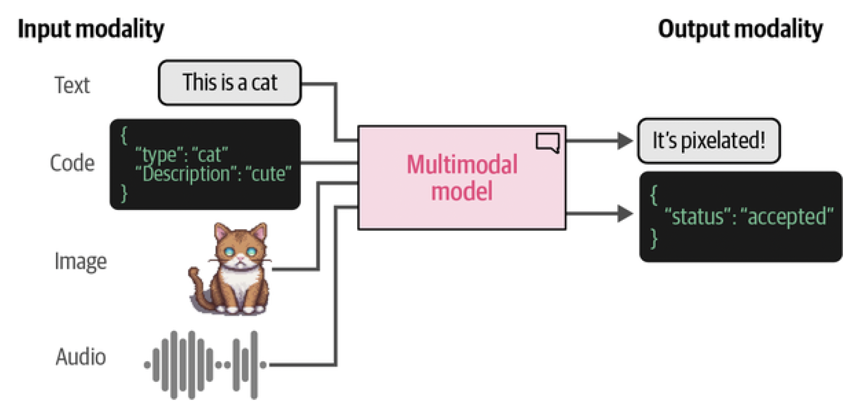
Figure 1. Models that are able to deal with different types (or modalities) of data, such as images, audio, video, or sensors, are said to be multimodal. It’s possible for a model to accept a modality as input yet not be able to generate in that modality.

We have seen all manner of emerging behaviors rising from LLMs, from generalization capabilities and reasoning to arithmetic and linguistics. As models grow larger and smarter, so do their skill sets.¹

The ability to receive and reason with multimodal input might further increase and help emerge capabilities that were previously locked. In practice, language does not solely live in a vacuum. As an example, your body language, facial expressions, intonation, etc. are all methods of communication that enhance the spoken word. The same thing applies to LLMs; if we can enable them to reason about multimodal information, their capabilities might increase and we become able to deploy them to solve new kinds of problems.

We will explore a number of different LLMs that have multimodal capabilities and what that means for practical use cases. We will start by exploring how images are converted to numerical representations using an adaptation of the original Transformer technique. Then, we will show how LLMs can be extended to include vision tasks using this Transformer.

Table of Contents

• Transformers for Vision
• Multimodal Embedding Models
  • CLIP: Connecting Text and Images
  • How Can CLIP Generate Multimodal Embeddings?
  • OpenCLIP
    • USING SENTENCE-TRANSFORMERS TO LOAD CLIP
• Making Text Generation Models Multimodal
  • BLIP-2: Bridging the Modality Gap
  • Preprocessing images
  • Preprocessing text
  • Use Case 1: Image Captioning
  • Use Case 2: Multimodal Chat-Based Prompting
• References

Transformers for Vision

Throughout the post, we have seen the success of using Transformer-based models for a variety of language modeling tasks, from classification and clustering to search and generative modeling. So it might not be surprising that researchers have been looking at a way to generalize some of the Transformer’s success to the field of computer vision. The method they came up with is called the Vision Transformer (ViT), which has been shown to do tremendously well on image recognition tasks compared to the previously default convolutional neural networks (CNNs).² Like the original Transformer, ViT is used to transform unstructured data, an image, into representations that can be used for a variety of tasks, like classification, as illustrated in Figure 2. ViT relies on an important component of the Transformer architecture, namely the encoder. The encoder is responsible for converting textual input into numerical representations before being passed to the decoder. However, before the encoder can perform its duties, the textual input needs to be tokenized first, as is illustrated in Figure 3.

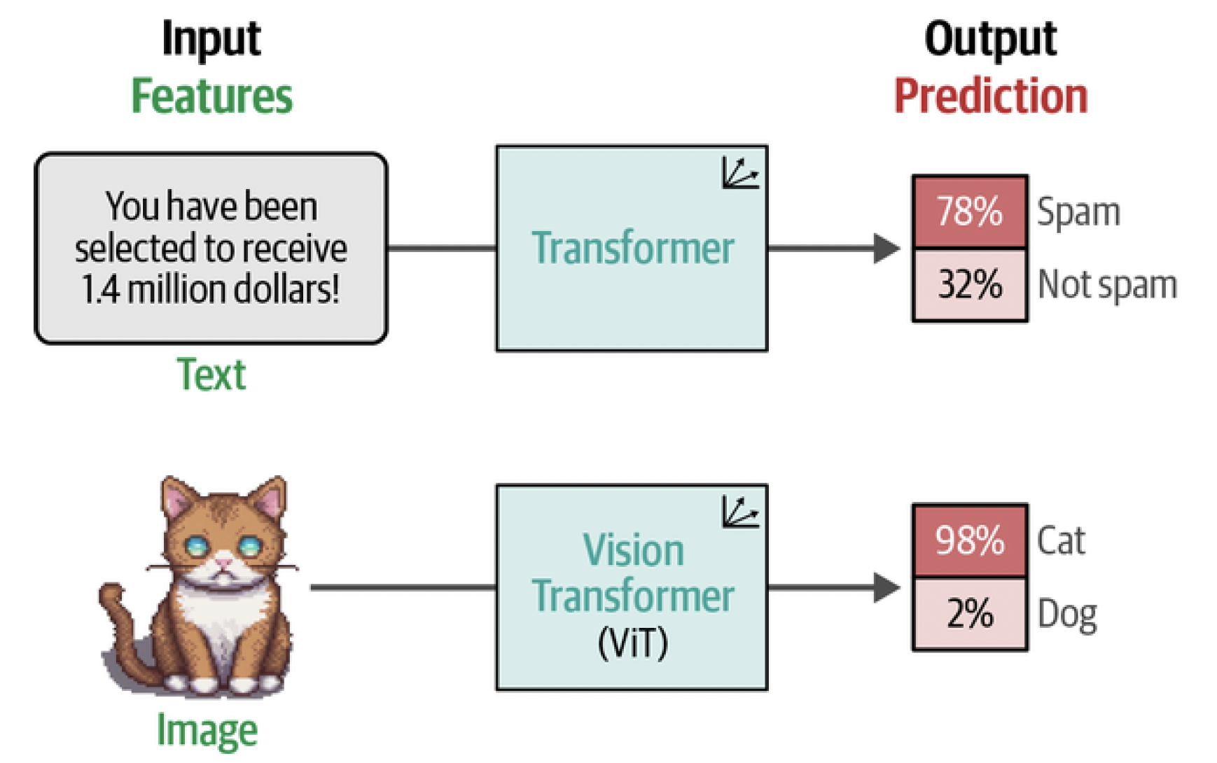
Figure 2. Both the original Transformer as well as the Vision Transformer take unstructured data, convert it to numerical representations, and finally use that for tasks like classification.

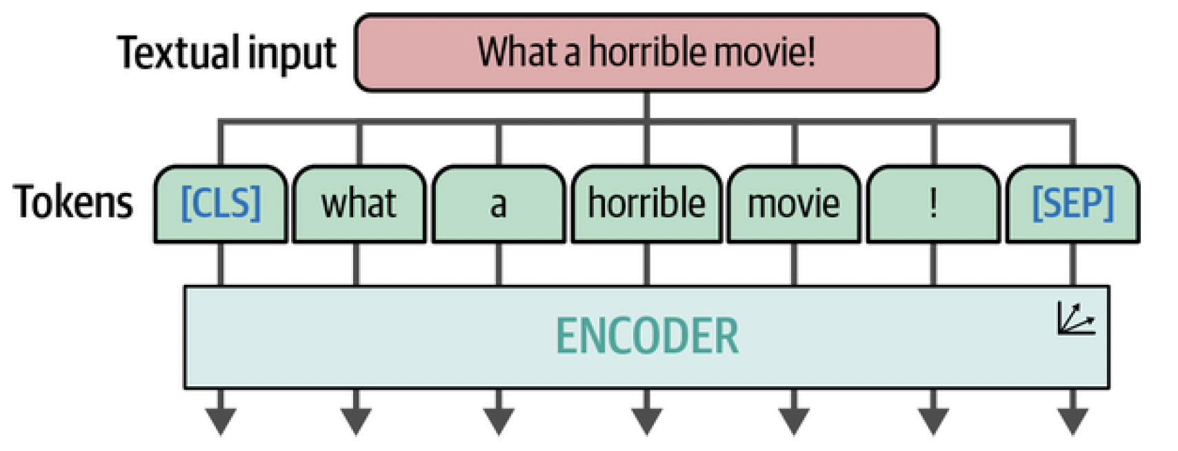
Figure 3. Text is passed to one or multiple encoders by first tokenizing it using a tokenizer.

Since an image does not consist of words this tokenization process cannot be used for visual data. Instead, the authors of ViT came up with a method for tokenizing images into "words," which allowed them to use the original encoder structure. Imagine that you have an image of a cat. This image is represented by a number of pixels, let’s say 512 × 512 pixels. Each individual pixel does not convey much information but when you combine patches of pixels, you slowly start to see more information. ViT uses a principle much like that. Instead of splitting up text into tokens, it converts the original image into patches of images. In other words, it cuts the image into a number of pieces horizontally and vertically as illustrated in Figure 4.

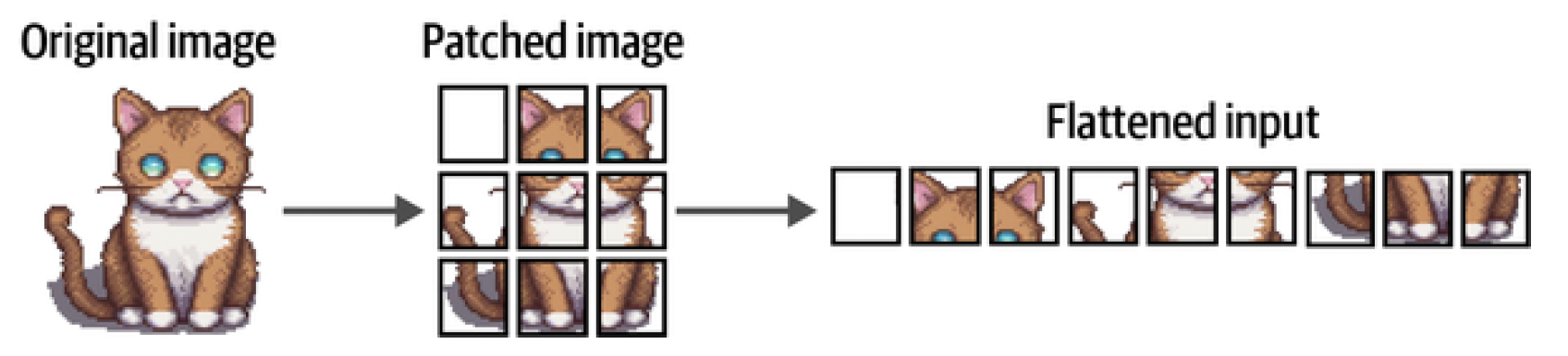
Figure 4. The "tokenization" process for image input. It converts an image into patches of subimages.

Just like we are converting text into tokens of text, we are converting an image into patches of images. The flattened input of image patches can be thought of as the tokens in a piece of text. However, unlike tokens, we cannot just assign each patch with an ID since these patches will rarely be found in other images, unlike the vocabulary of a text. Instead, the patches are linearly embedded to create numerical representations, namely embeddings. These can then be used as the input of a Transformer model. That way, the patches of images are treated the same way as tokens. The full process is illustrated in Figure 5. For illustrative purposes, the images in the examples were patched into 3 × 3 patches but the original implementation used 16 × 16 patches. After all, the paper is called "An Image is Worth 16x16 Words." What is so interesting about this approach is that the moment the embeddings are passed to the encoder, they are treated as if they were textual tokens. From that point forward, there is no difference in how a text or image trains. Due to these similarities, the ViT is often used to make all kinds of language models multimodal. One of the most straightforward ways to use it is during the training of embedding models.

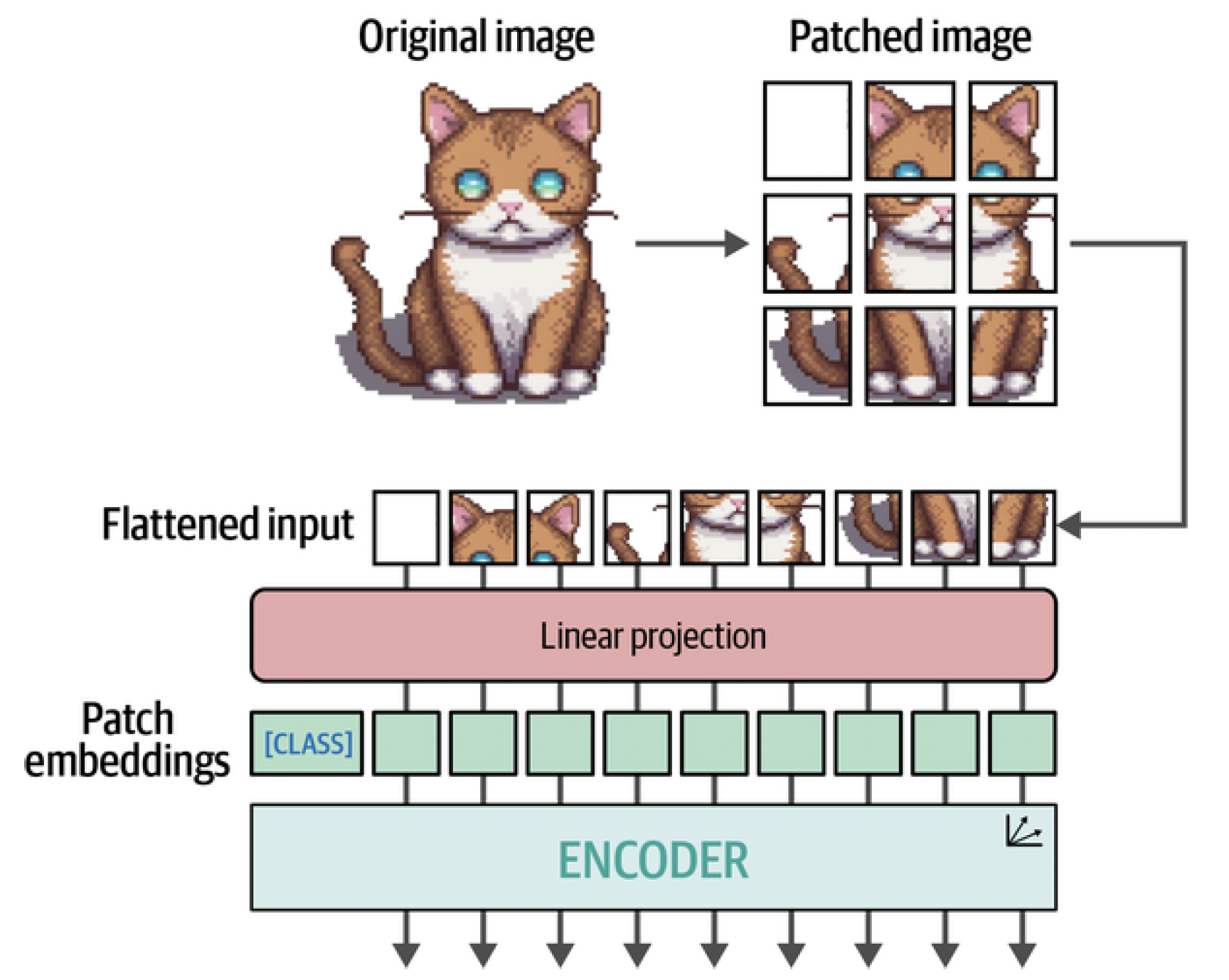
Figure 5. The main algorithm behind ViT. After patching the images and linearly projecting them, the patch embeddings are passed to the encoder and treated as if they were textual tokens.

Multimodal Embedding Models

We used embedding models to capture the semantic content of textual representations, such as papers and documents. We saw that we could use these embeddings or numerical representations to find similar documents, apply classification tasks, and even perform topic modeling. As we have seen many times before, embeddings often are an important driver behind LLM applications. They are an efficient method for capturing large-scale information and searching for the needle in the haystack of information. That said, we have looked at text-only embedding models thus far, which focus on generating embeddings for textual representations. Although embedding models exist for solely embedding imagery, we will look at embedding models that can capture both textual as well as visual representations. We illustrate this in Figure 6.

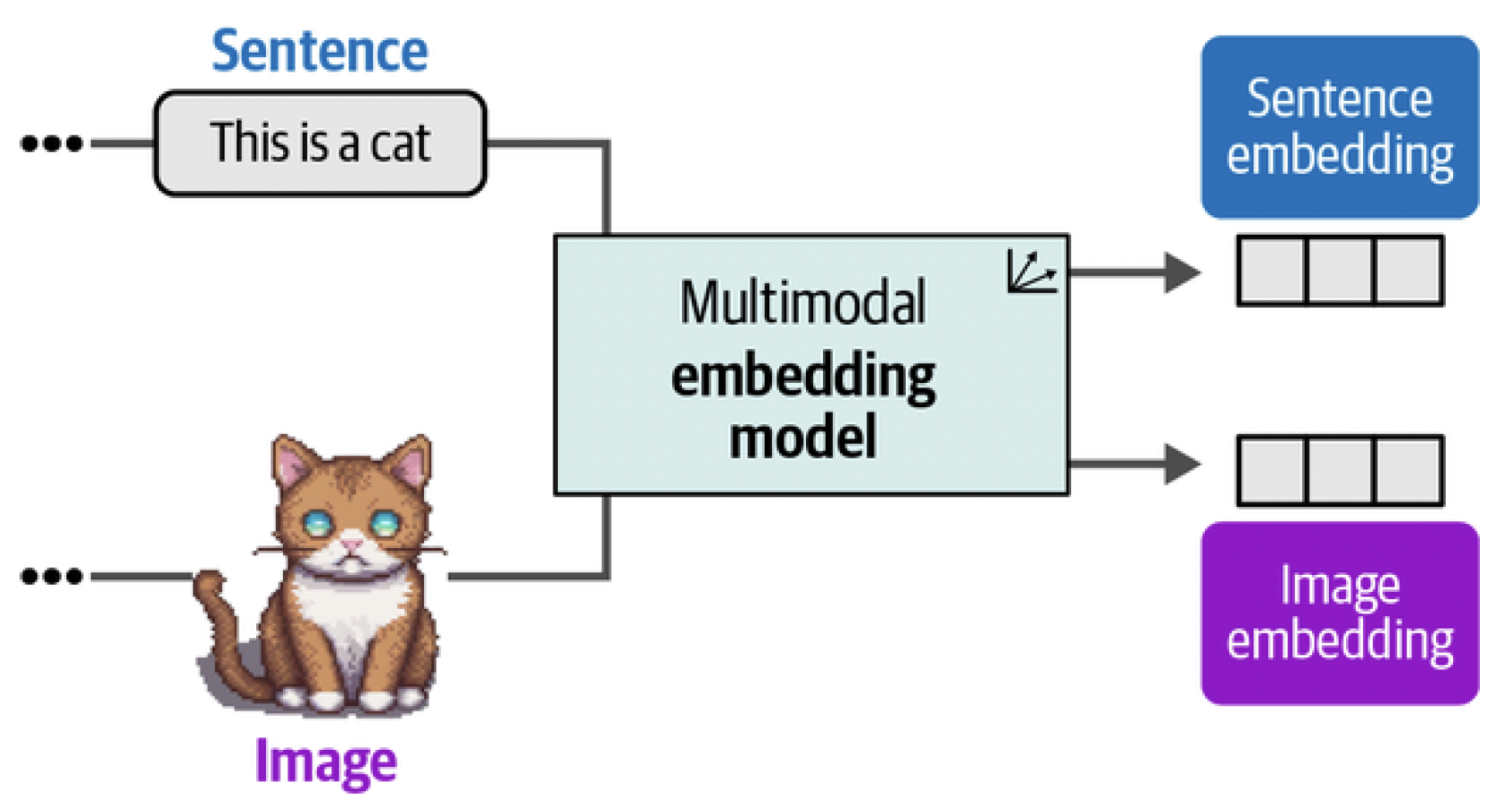
Figure 6. Multimodal embedding models can create embeddings for multiple modalities in the same vector space.

An advantage is that this allows for comparing multimodal representations since the resulting embeddings lie in the same vector space (Figure 7). For instance, using such a multimodal embedding model, we can find images based on input text. What images would we find if we search for images similar to "pictures of a puppy"? Vice versa would also be possible. Which documents are best related to this question?

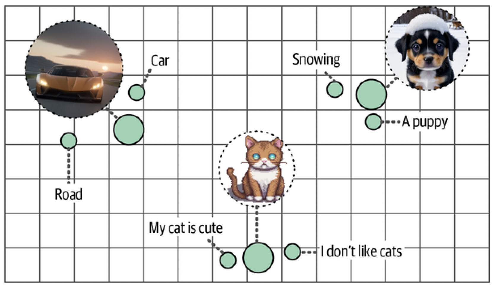
Figure 7. Despite having coming from different modalities, embeddings with similar meaning will be close to each other in vector space.

There are a number of multimodal embedding models, but the most well- known and currently most-used model is Contrastive Language-Image Pre- training (CLIP).

CLIP: Connecting Text and Images

CLIP is an embedding model that can compute embeddings of both images and texts. The resulting embeddings lie in the same vector space, which means that the embeddings of images can be compared with the embeddings of text.³ This comparison capability makes CLIP, and similar models, usable for tasks such as:

• Zero-shot classification: We can compare the embedding of an image with that of the description of its possible classes to find which class is most similar.
• Clustering: Cluster both images and a collection of keywords to find which keywords belong to which sets of images.
• Search: Across billions of texts or images, we can quickly find what relates to an input text or image.
• Generation: Use multimodal embeddings to drive the generation of images (e.g., stable diffusion⁴).

How Can CLIP Generate Multimodal Embeddings?

The procedure of CLIP is actually quite straightforward. Imagine that you have a dataset with millions of images alongside captions as we illustrate in Figure 8.

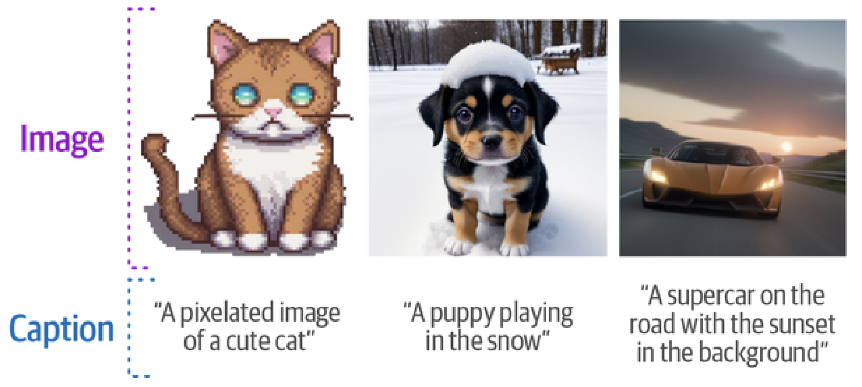
Figure 8. The type of data that is needed to train a multimodal embedding model.

This dataset can be used to create two representations for each pair, the image and its caption. To do so, CLIP uses a text encoder to embed text and an image encoder to embed images. As is shown in Figure 9, the result is an embedding for both the image and its corresponding caption.

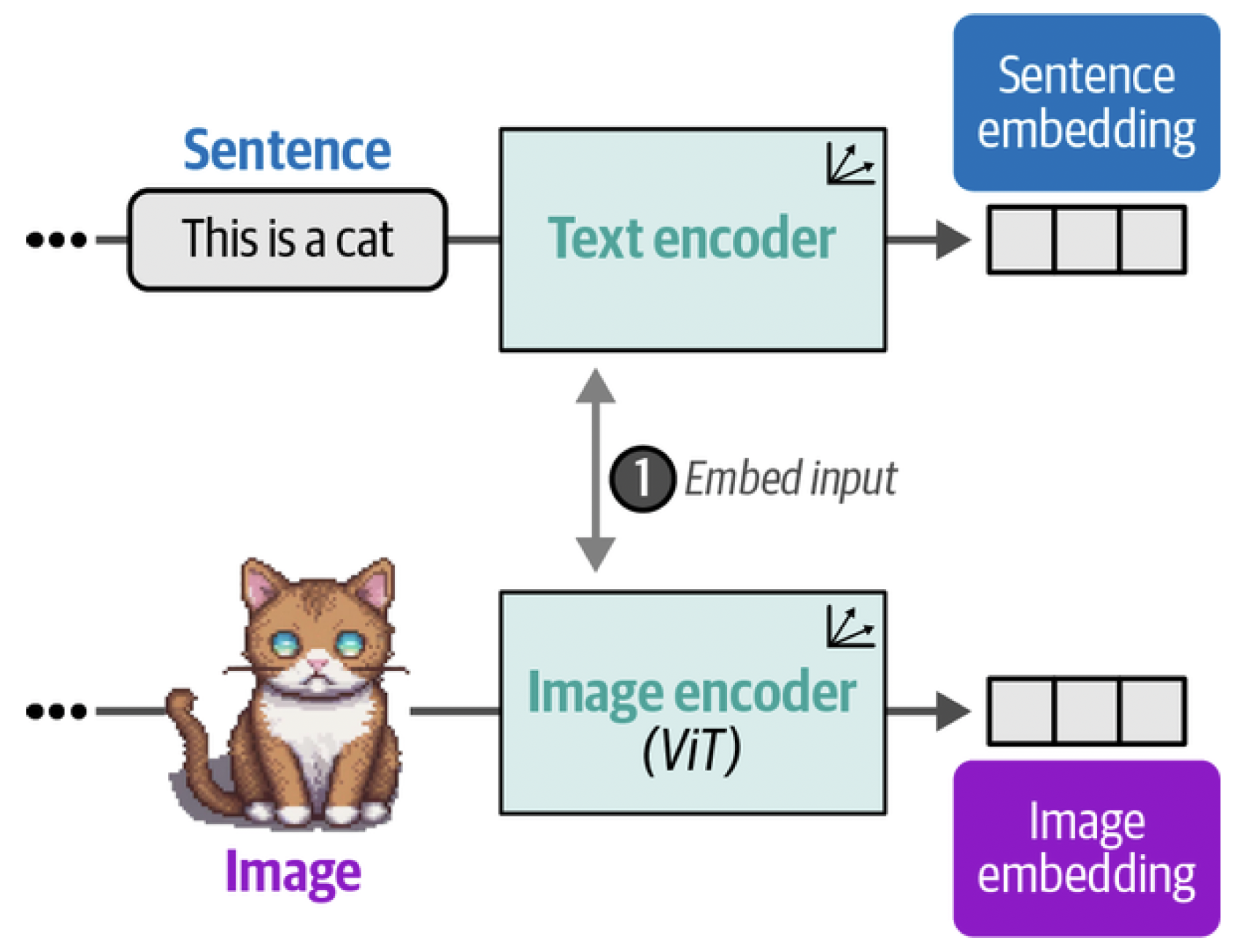
Figure 9. In the first step of training CLIP, both images and text are embedded using an image and text encoder, respectively.

The pair of embeddings that are generated are compared through cosine similarity. Cosine similarity is the cosine of the angle between vectors, which is calculated through the dot product of the embeddings and divided by the product of their lengths. When we start training, the similarity between the image embedding and text embedding will be low as they are not yet optimized to be within the same vector space. During training, we optimize for the similarity between the embeddings and want to maximize them for similar image/caption pairs and minimize them for dissimilar image/caption pairs (Figure 10). After calculating their similarity, the model is updated and the process starts again with new batches of data and updated representations (Figure 11). This method is called contrastive learning.

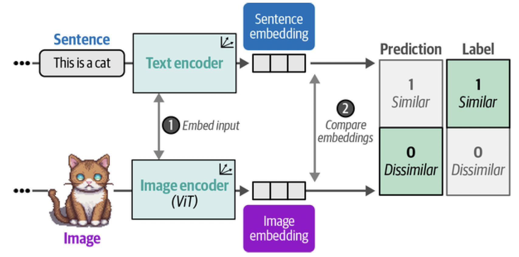
Figure 10. In the second step of training CLIP, the similarity between the sentence and image embedding is calculated using cosine similarity.

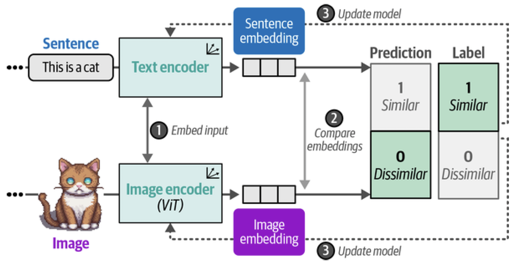
Figure 11. In the third step of training CLIP, the text and image encoders are updated to match what the intended similarity should be. This updates the embeddings such that they are closer in vector space if the inputs are similar.

Eventually, we expect the embedding of an image of a cat would be similar to the embedding of the phrase "a picture of a cat." As we will see in theory of contrastive learning, to make sure the representations are as accurate as possible, negative examples of images and captions that are not related should also be included in the training process. Modeling similarity is not only knowing what makes things similar to one another, but also what makes them different and dissimilar.

OpenCLIP

For our next example, we are going to be using models from the open source variant of CLIP, namely OpenCLIP. Using OpenCLIP, or any CLIP model, boils down to two things: processing the textual and image inputs before passing them to the main model. Before doing so, let’s take a look at a small example where we will be using one of the images we have seen before, namely, an AI-generated image (through stable diffusion) of a puppy playing in the snow, as illustrated in Figure 12:

from urllib.request import urlopen
from PIL import Image

# Load an AI-generated image of a puppy playing in the snow
puppy_path = "puppy.png"
image = Image.open(urlopen(puppy_path)).convert("RGB")

caption = "a puppy playing in the snow"

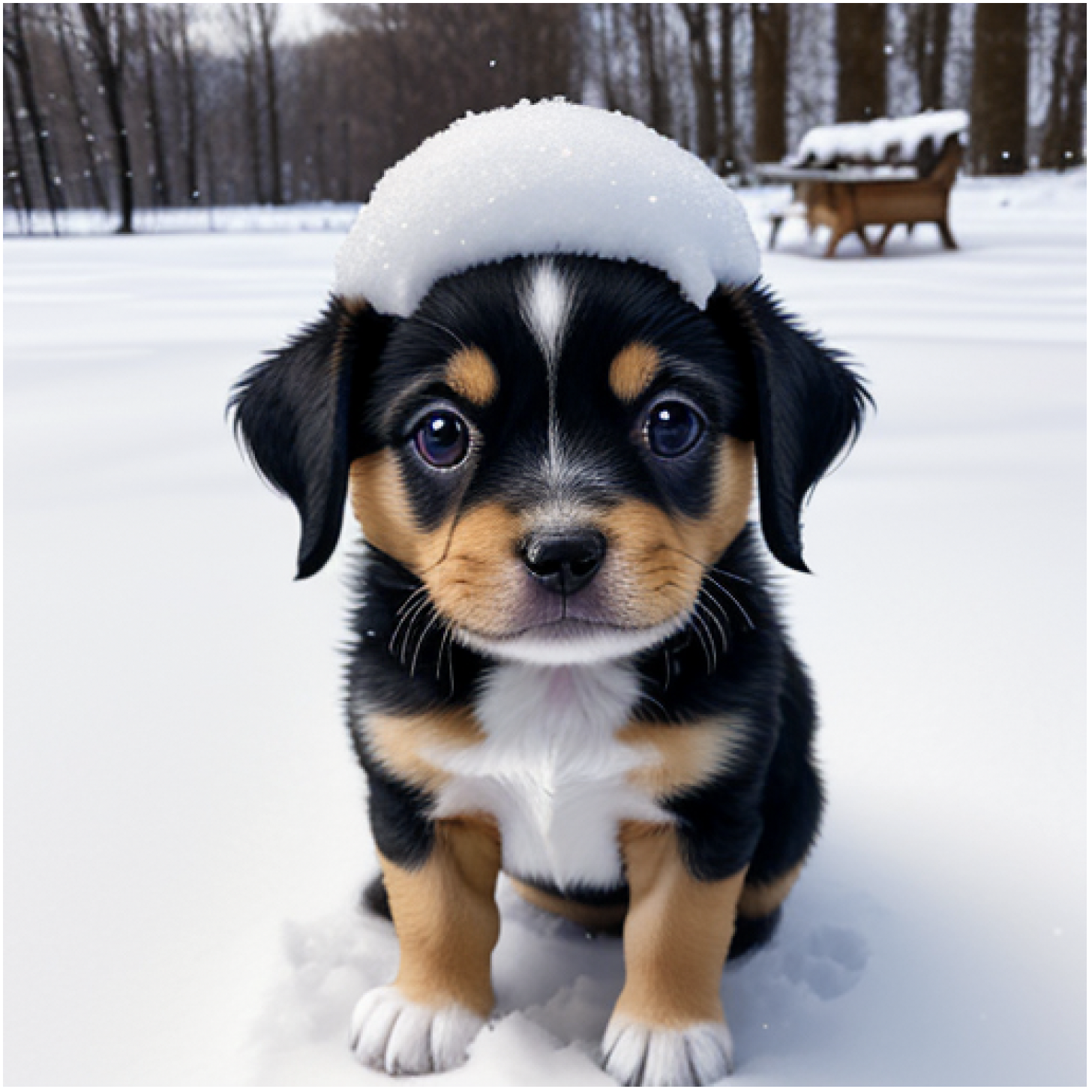
Figure 12. An AI-generated image of a puppy playing in the snow.

Since we have a caption for this image, we can use OpenCLIP to generate embeddings for both. To do so, we load in three models: A tokenizer for tokenizing the textual input A preprocessor to preprocess and resize the image The main model that converts the previous outputs to embeddings

from transformers import CLIPTokenizerFast, CLIPProcessor, CLIPModel

model_id = "openai/clip-vit-base-patch32"

# Load a tokenizer to preprocess the text
clip_tokenizer = CLIPTokenizerFast.from_pretrained(model_id)

# Load a processor to preprocess the images
clip_processor = CLIPProcessor.from_pretrained(model_id)

# Main model for generating text and image embeddings
model = CLIPModel.from_pretrained(model_id)

After having loaded in the models, preprocessing our input is straightforward. Let’s start with the tokenizer and see what happens if we preprocess our input:

# Tokenize our input
inputs = clip_tokenizer(caption, return_tensors="pt")
inputs

This outputs a dictionary that contains the IDs of the input:

{'input_ids': tensor([[49406, 320, 6829, 1629, 530, 518, 2583, 49407]]), 'attention_mask': tensor([[1, 1, 1, 1, 1, 1, 1, 1]])}

To see what those IDs represent, we can convert them to tokens using the aptly named convert_ids_to_tokens function:

# Convert our input back to tokens
clip_tokenizer.convert_ids_to_tokens(inputs["input_ids"][ 0 ])

This gives us the following output:

['<|startoftext|>',
'a</w>',
'puppy</w>',
'playing</w>',
'in</w>',
'the</w>',
'snow</w>',
'<|endoftext|>']

As we often have seen before, the text is split up into tokens. Additionally, we now also see that the start and end of the text is indicated to separate it from a potential image embedding. You might also notice that the [CLS] token is missing. In CLIP, the [CLS] token is actually used to represent the image embedding. Now that we have preprocessed our caption, we can create the embedding:

# Create a text embedding
text_embedding = model.get_text_features(**inputs)
text_embedding.shape

This results in an embedding that has 512 values for this single string:

torch.Size([1, 512])

Before we can create our image embedding, like the text embedding, we will need to preprocess it as the model expects the input image to have certain characteristics, like its size and shape. To do so, we can use the processor that we created before:

# Preprocess image
processed_image = clip_processor(text=None, images=image, return_tensors="pt")["pixel_values"]
processed_image.shape

The original image was 512 × 512 pixels. Notice that the preprocessing of this image reduced its size to 224 × 224 pixels as that is its expected size:

torch.Size([1, 3, 224, 224])

Let’s visualize the results of this preprocessing as shown in Figure 13:

import torch
import numpy as np
import matplotlib.pyplot as plt

# Prepare image for visualization
img = processed_image.squeeze( 0 )
img = img.permute(*torch.arange(img.ndim - 1, -1, -1 ))
img = np.einsum("ijk->jik", img)

# Visualize preprocessed image
plt.imshow(img)
plt.axis("off")

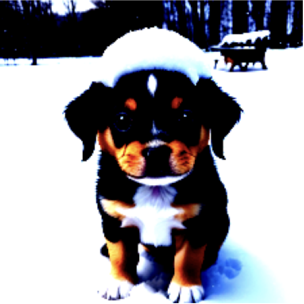
Figure 13. The preprocessed input image by CLIP.

To convert this preprocessed image into embeddings, we can call the model as we did before and explore what shape it returns:

# Create the image embedding
image_embedding = model.get_image_features(processed_image)
image_embedding.shape

This gives us the following shape:

torch.Size([1, 512])

Notice that the shape of the resulting image embedding is the same as that of the text embedding. This is important as it allows us to compare their embeddings and see if they are similar. We can use these embeddings to calculate how similar they are. To do so, we normalize the embeddings first before calculating the dot product to give us a similarity score:

# Normalize the embeddings
text_embedding /= text_embedding.norm(dim=-1, keepdim=True)
image_embedding /= image_embedding.norm(dim=-1, keepdim=True)

# Calculate their similarity
text_embedding = text_embedding.detach().cpu().numpy()
image_embedding = image_embedding.detach().cpu().numpy()
score = np.dot(text_embedding, image_embedding.T)
score

This gives us the following score:

array([[0.33149648]], dtype=float32)

We get a similarity score of 0.33, which is difficult to interpret considering we don’t know what the model considers a low versus a high similarity score. Instead, let’s extend the example with more images and captions as illustrated in Figure 14.

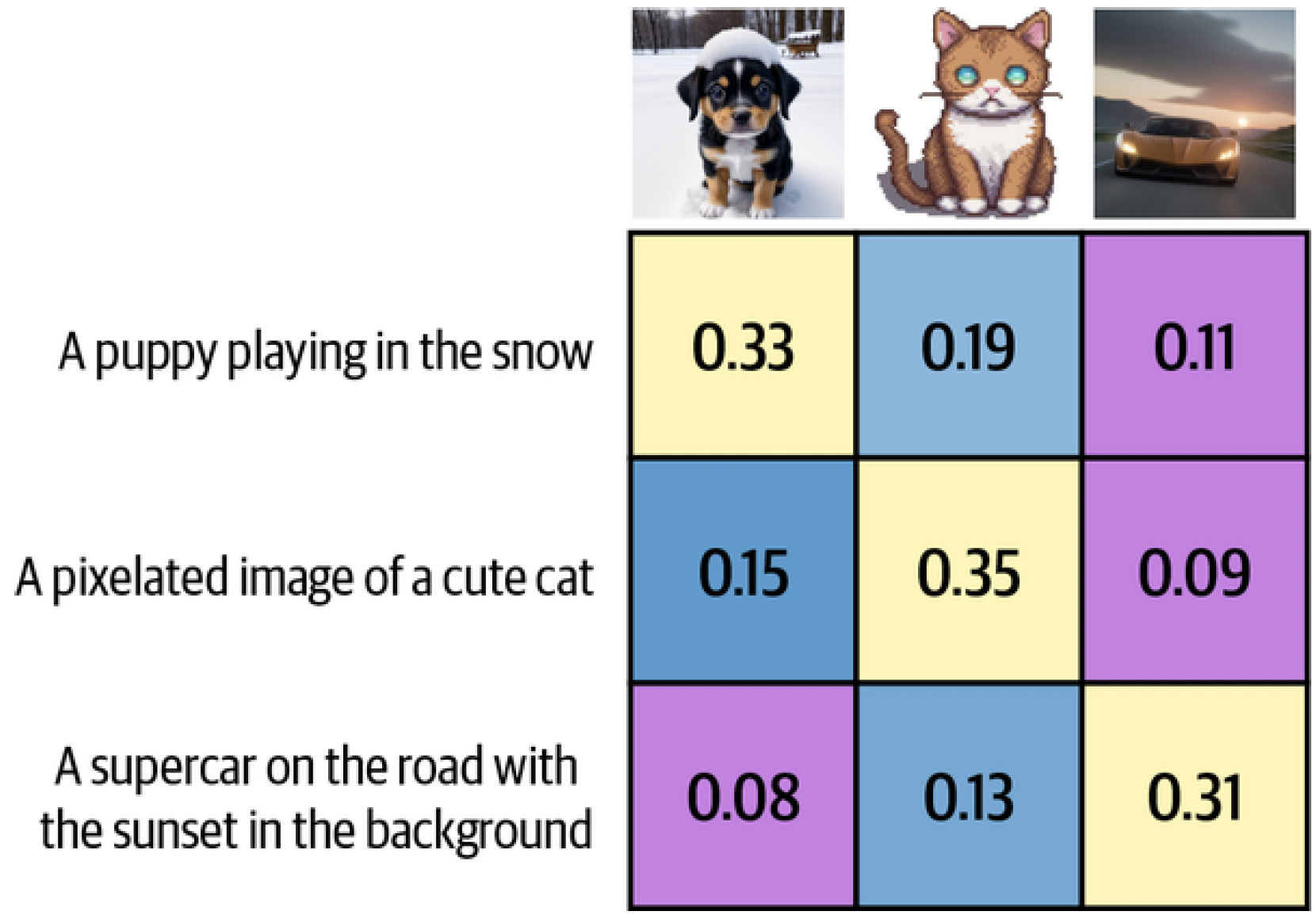
Figure 14. The similarity matrix between three images and three captions.

It seems that a score of 0.33 is indeed high considering the similarities with other images are quite a bit lower.

USING SENTENCE-TRANSFORMERS TO LOAD CLIP

sentence-transformers implements a few CLIP-based models that make it much easier to create embeddings. It only takes a few lines of code:

from sentence_transformers import SentenceTransformer, util

# Load SBERT-compatible CLIP model
model = SentenceTransformer("clip-ViT-B-32")

# Encode the images
image_embeddings = model.encode(images)

# Encode the captions
text_embeddings = model.encode(captions)

#Compute cosine similarities
sim_matrix = util.cos_sim(image_embeddings, text_embeddings)

Making Text Generation Models Multimodal

Traditionally, text generation models have been, as you might expect, models that interpret textual representations. Models like Llama 2 and ChatGPT excel at reasoning about textual information and responding with natural language. They are, however, limited to the modality they were trained in, namely text. As we have seen before with multimodal embedding models, the addition of vision can enhance the capabilities of a model. In the case of text generation models, we would like it to reason about certain input images. For example, we could give it an image of a pizza and ask it what ingredients it contains. You could show it a picture of the Eiffel Tower and ask when it was built or where it is located. This conversational ability is further illustrated in Figure 15.

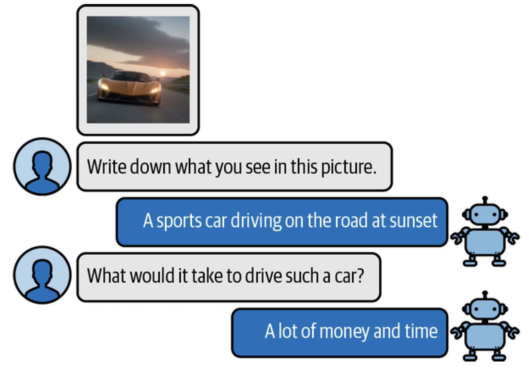
Figure 15. An example of a multimodal text generation model (BLIP-2) that can reason about input images.

To bridge the gap between these two domains, attempts have been made to introduce a form of multimodality to existing models. One such method is called BLIP-2: Bootstrapping Language-Image Pre-training for Unified Vision-Language Understanding and Generation 2. BLIP-2 is an easy-to- use and modular technique that allows for introducing vision capabilities to existing language models.

BLIP-2: Bridging the Modality Gap

Creating a multimodal language model from scratch requires significant computing power and data. We would have to use billions of images, text, and image-text pairs to create such a model. As you can imagine, this is not easily feasible!

Instead of building the architecture from scratch, BLIP-2 bridges the vision-language gap by building a bridge, named the Querying Transformer (Q- Former), that connects a pretrained image encoder and a pretrained LLM.⁵ By leveraging pretrained models, BLIP-2 only needs to train the bridge without needing to train the image encoder and LLM from scratch. It makes great use of the technology and models that are already out there! This bridge is illustrated in Figure 16.

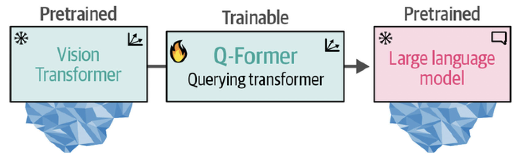
Figure 16. The Querying Transformer is the bridge between vision (ViT) and text (LLM) that is the only trainable component of the pipeline.

To connect the two pretrained models, the Q-Former mimics their architectures. It has two modules that share their attention layers: An Image Transformer to interact with the frozen Vision Transformer for feature extraction A Text Transformer that can interact with the LLM The Q-Former is trained in two stages, one for each modality, as illustrated in Figure 17. In step 1, image-document pairs are used to train the Q-Former to represent both images and text. These pairs are generally captions of images, as we have seen before when training CLIP. The images are fed to the frozen ViT to extract vision embeddings. These embeddings are used as the input of Q-Former’s ViT. The captions are used as the input of Q-Former’s Text Transformer.

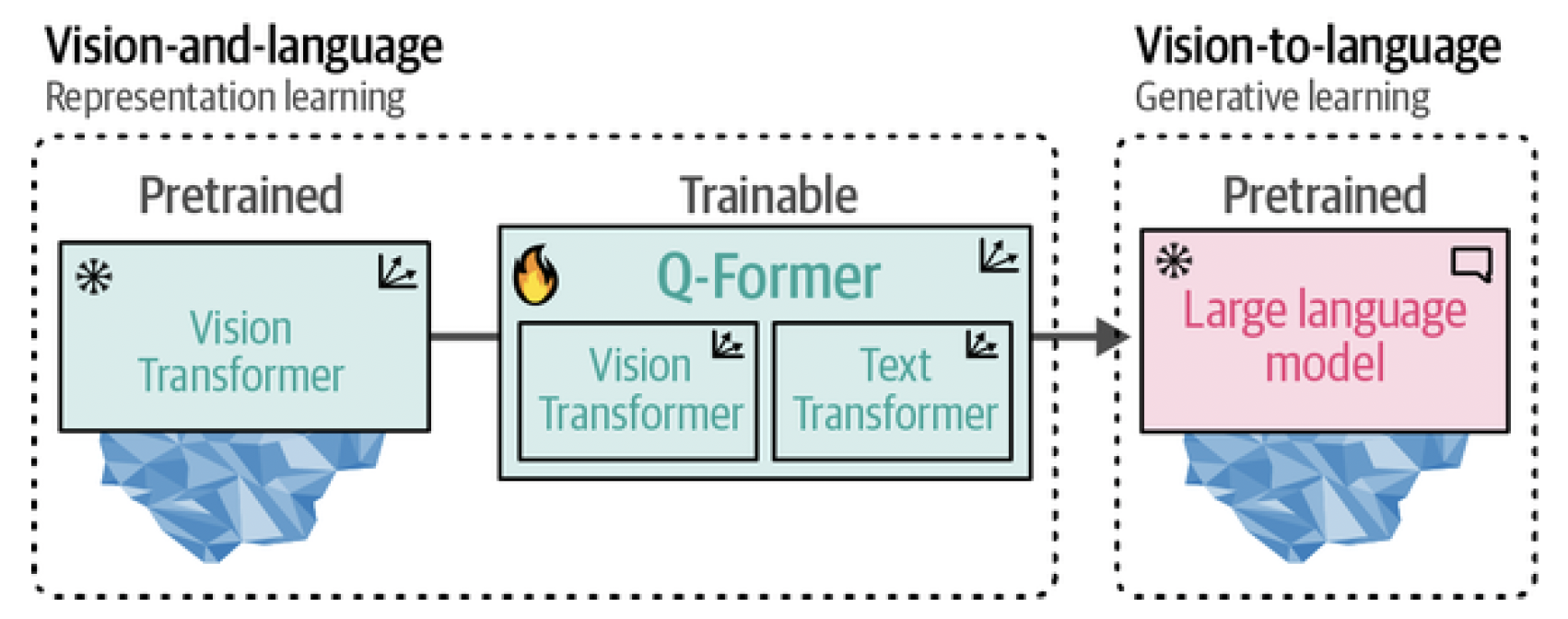
Figure 17. In step 1, representation learning is applied to learn representations for vision and language simultaneously. In step 2, these representations are converted to soft visual prompts to feed the LLM.

With these inputs, the Q-Former is then trained on three tasks: Image-text contrastive learning This task attempts to align pairs of image and text embeddings such that they maximize their mutual information. Image-text matching A classification task to predict whether an image and text pair is positive (matched) or negative (unmatched). Image-grounded text generation Trains the model to generate text based on information extracted from the input image. These three objectives are jointly optimized to improve the visual representations that are extracted from the frozen ViT. In a way, we are trying to inject textual information into the embeddings of the frozen ViT so that we can use them in the LLM. This first step of BLIP-2 is illustrated in Figure 18.

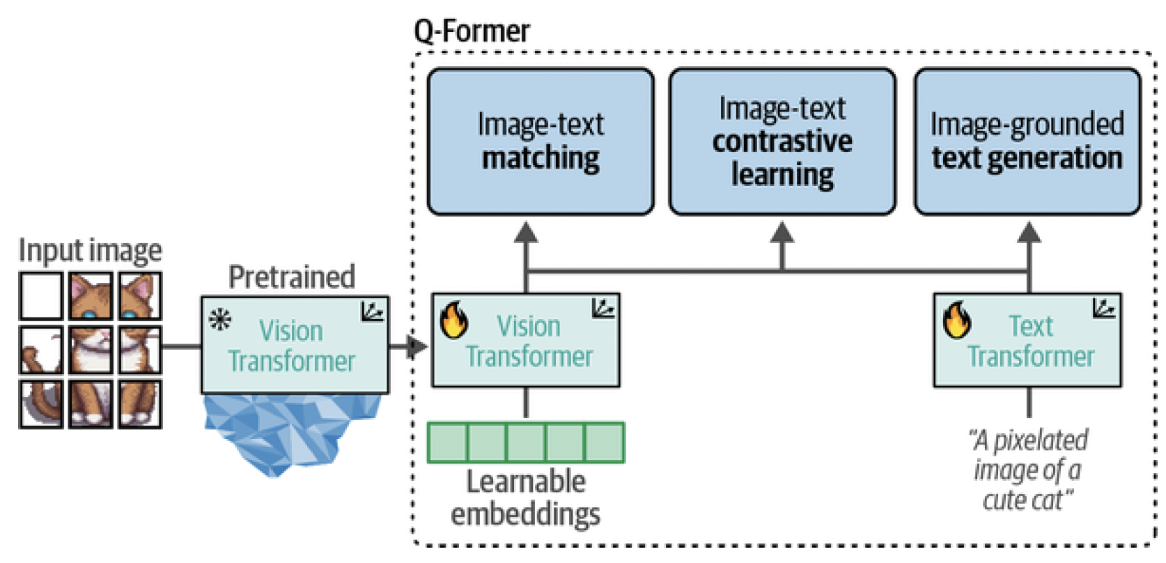
Figure 18. In step 1, the output of the frozen ViT is used together with its caption and trained on three contrastive-like tasks to learn visual-text representations.

In step 2, the learnable embeddings derived from step 1 now contain visual information in the same dimensional space as the corresponding textual information. The learnable embeddings are then passed to the LLM. In a way, these embeddings serve as soft visual prompts that condition the LLM on the visual representations that were extracted by the Q-Former. There is also a fully connected linear layer in between them to make sure that the learnable embeddings have the same shape as the LLM expects. This second step of converting vision to language is represented in Figure 19.

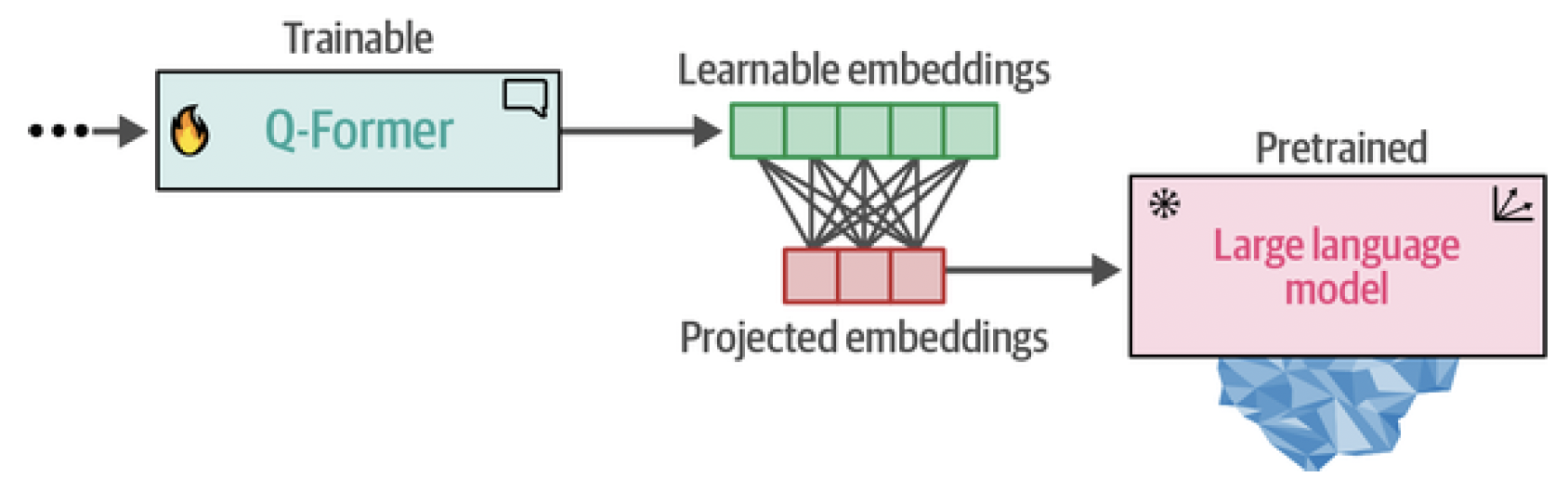
Figure 19. In step 2, the learned embeddings from the Q-Former are passed to the LLM through a projection layer. The projected embeddings serve as a soft visual prompt.

When we put these steps together, they make it possible for the Q-Former to learn visual and textual representations in the same dimensional space, which can be used as a soft prompt to the LLM. As a result, the LLM will be given information about the image in a similar manner to the context you would provide an LLM when prompting. The full in-depth process is illustrated in Figure 20.

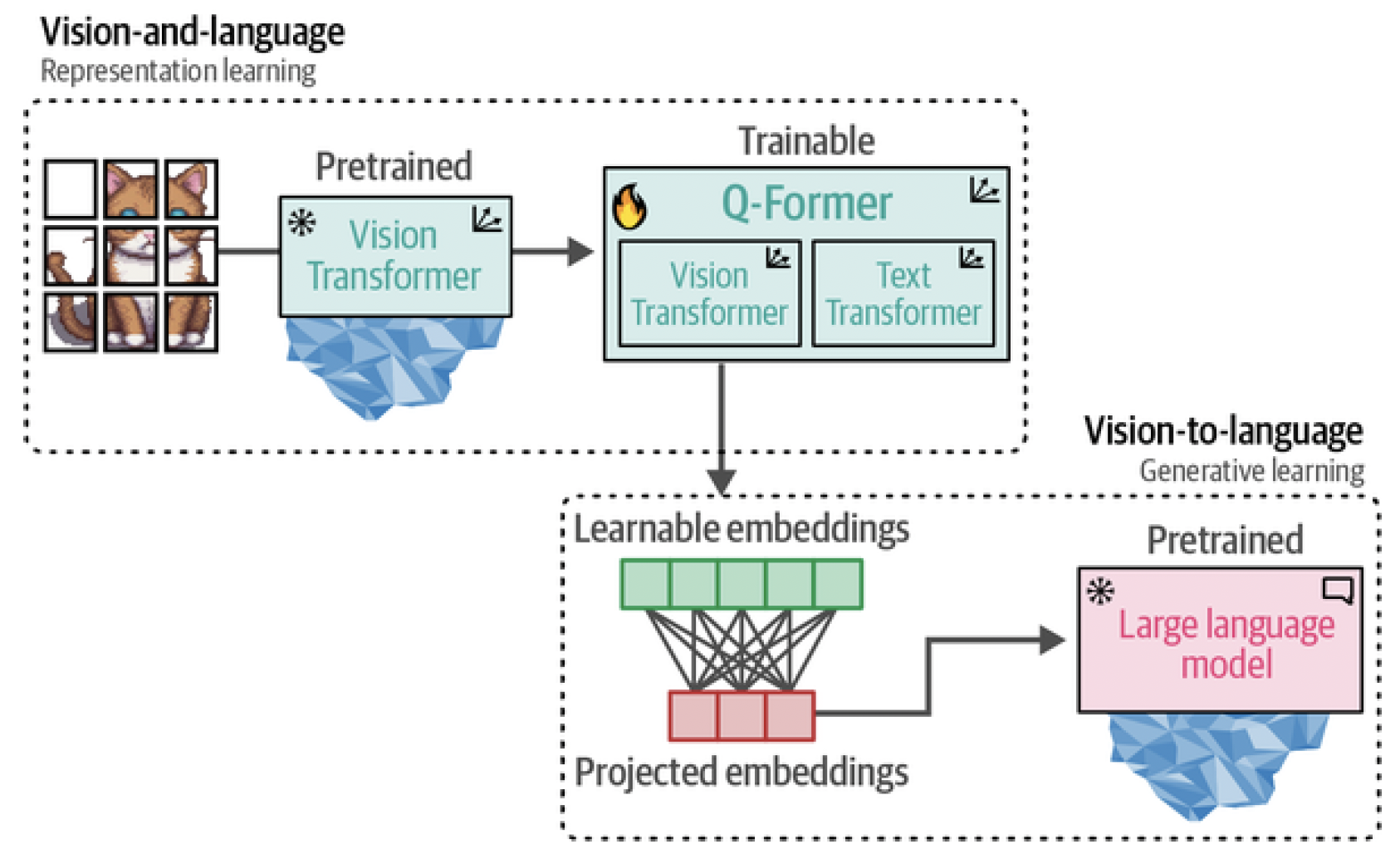Figure 20. The full BLIP-2 procedure.

Since BLIP-2, many other visual LLMs have been released that have similar processes, like LLaVA, a framework for making textual LLMs multimodal⁶ or Idefics 2, an efficient visual LLM based on the Mistral 7B LLM.⁷ Both visual LLMs, although having different architectures, connect pretrained CLIP-like visual encoders with textual LLMs. The goal of these architectures is to project visual features from the input images to language embeddings such that they can be used as the input for an LLM. Similar to the Q-Former, they attempt to bridge the gap between images and text.

Preprocessing Multimodal Inputs Now that we know how BLIP-2 is created, there are a number of interesting use cases for such a model, not limited to captioning images, answering visual questions, and even performing prompting. Before we go through some use cases, let’s first load the model and explore how you can use it:

from transformers import AutoProcessor, Blip2ForConditionalGeneration
import torch

# Load processor and main model
blip_processor = AutoProcessor.from_pretrained("Salesforce/blip2-opt-2.7b")
model = Blip2ForConditionalGeneration.from_pretrained("Salesforce/blip2-opt-2.7b", torch_dtype=torch.float16)

# Send the model to GPU to speed up inference
device = "cuda" if torch.cuda.is_available() else "cpu"
model.to(device)

TIP: Using model.vision_model and model.language_model, we can see which ViT and generative model are used, respectively, in the BLIP-2 model we loaded.

We loaded two components that make up our full pipeline: a processor and a model. The processor can be compared to the tokenizer of language models. It converts unstructured input, such as images and text, to representations that the model generally expects.

Preprocessing images

Let’s start by exploring what the processor does to images. We start by loading the picture of a very wide image for illustration purposes:

# Load image of a supercar
car_path = "car.png"
image = Image.open(urlopen(car_path)).convert("RGB")

image

The image has 520 × 492 pixels, which is generally an unusual format. So let’s see what our processor does to it:

# Preprocess the image
inputs = blip_processor(image, return_tensors="pt").to(device, torch.float16)
inputs["pixel_values"].shape

This gives us the following shape:

torch.Size([1, 3, 224, 224])

The result is a 224 × 224-sized image. Quite a bit smaller than we initially had! This also means that all the original different shapes of the image will be processed into squares. So be careful inputting very wide or tall images as they might get distorted.

Preprocessing text

Let’s continue this exploration of the processor with text instead. First, we can access the tokenizer used to tokenize the input text:

blip_processor.tokenizer

This gives us the following output:

GPT2TokenizerFast(name_or_path='Salesforce/blip2-opt-2.7b',
vocab_size=50265,
model_max_length=1000000000000000019884624838656, is_fast=True,
padding_side='right', truncation_side='right', special_tokens=
{'bos_token': '</s>', 'eos_token': '</s>', 'unk_token': '</s>',
'pad_token': '<pad>'}, clean_up_tokenization_spaces=True),
added_tokens_decoder={
1: AddedToken("<pad>", rstrip=False, lstrip=False,
single_word=False, normalized=True, special=True),
2: AddedToken("</s>", rstrip=False, lstrip=False,
single_word=False, normalized=True, special=True),
}

The BLIP-2 model here uses a GPT2Tokenizer. To explore how GPT2Tokenizer works, we can try it out with a small sentence. We start by converting the sentence to token IDs before converting them back to tokens:

# Preprocess the text
text = "Her vocalization was remarkably melodic"
token_ids = blip_processor(image, text=text, return_tensors="pt")
token_ids = token_ids.to(device, torch.float16)["input_ids"][ 0 ]

# Convert input ids back to tokens
tokens =
blip_processor.tokenizer.convert_ids_to_tokens(token_ids)
tokens

This gives us the following tokens:

['</s>', 'Her', 'Ġvocal', 'ization', 'Ġwas', 'Ġremarkably', 'Ġmel', 'odic']

When we inspect the tokens, you might notice a strange symbol at the beginning of some tokens, namely, the Ġ symbol. This is actually supposed to be a space. However, an internal function takes characters in certain code points and moves them up by 256 to make them printable. As a result, the space (code point 32) becomes Ġ (code point 288).

We will convert them to underscores for illustrative purposes:

# Replace the space token with an underscore
tokens = [token.replace("Ġ", "_") for token in tokens]
tokens

This gives us a nicer output:

['</s>', 'Her', '_vocal', 'ization', '_was', '_remarkably', '_mel', 'odic']

The output shows that the underscore indicates the beginning of a word. That way, words that are made up of multiple tokens can be recognized.

Use Case 1: Image Captioning

The most straightforward usage of a model like BLIP-2 is to create captions of images that you have in your data. You might be a store that wants to create descriptions of its clothing or perhaps you are a photographer that does not have the time to manually label the 1,000+ pictures of a wedding. The process of captioning an image closely follows the processing. An image is converted to pixel values that the model can read. These pixel values are passed to BLIP-2 to be converted into soft visual prompts that the LLM can use to decide on a proper caption. Let’s take the image of a supercar and use the processor to derive pixels in the expected shape:

# Load an AI-generated image of a supercar
image = Image.open(urlopen(car_path)).convert("RGB")

# Convert an image into inputs and preprocess it
inputs = blip_processor(image, return_tensors="pt").to(device, torch.float16)
image

The next step is converting the image into token IDs using the BLIP-2 model. After doing so, we can convert the IDs into text (the generated caption):

# Generate image ids to be passed to the decoder (LLM)
generated_ids = model.generate(**inputs, max_new_tokens= 20 )

# Generate text from the image ids
generated_text = blip_processor.batch_decode(generated_ids, skip_special_tokens= True)
generated_text = generated_text[0].strip()
generated_text

generated_text contains the caption:

an orange supercar driving on the road at sunset

This seems like a perfect description for this image! Image captioning is a great way to get to learn this model before stepping into more complex use cases. Try it out with a few images yourself and see where it performs well and where it performs poorly. Domain-specific images, like pictures of specific cartoon characters or imaginary creations, may fail as the model was trained on largely public data. Let’s end this use case with a fun example, namely an image from the Rorschach test, which is illustrated in Figure 21. It is part of an old psychological experiment that tests the individual’s perception of inkblots.⁸ What someone sees in such an inkblot supposedly tells you something about a person’s personality characteristics. It is quite a subjective test but that just makes it more fun!

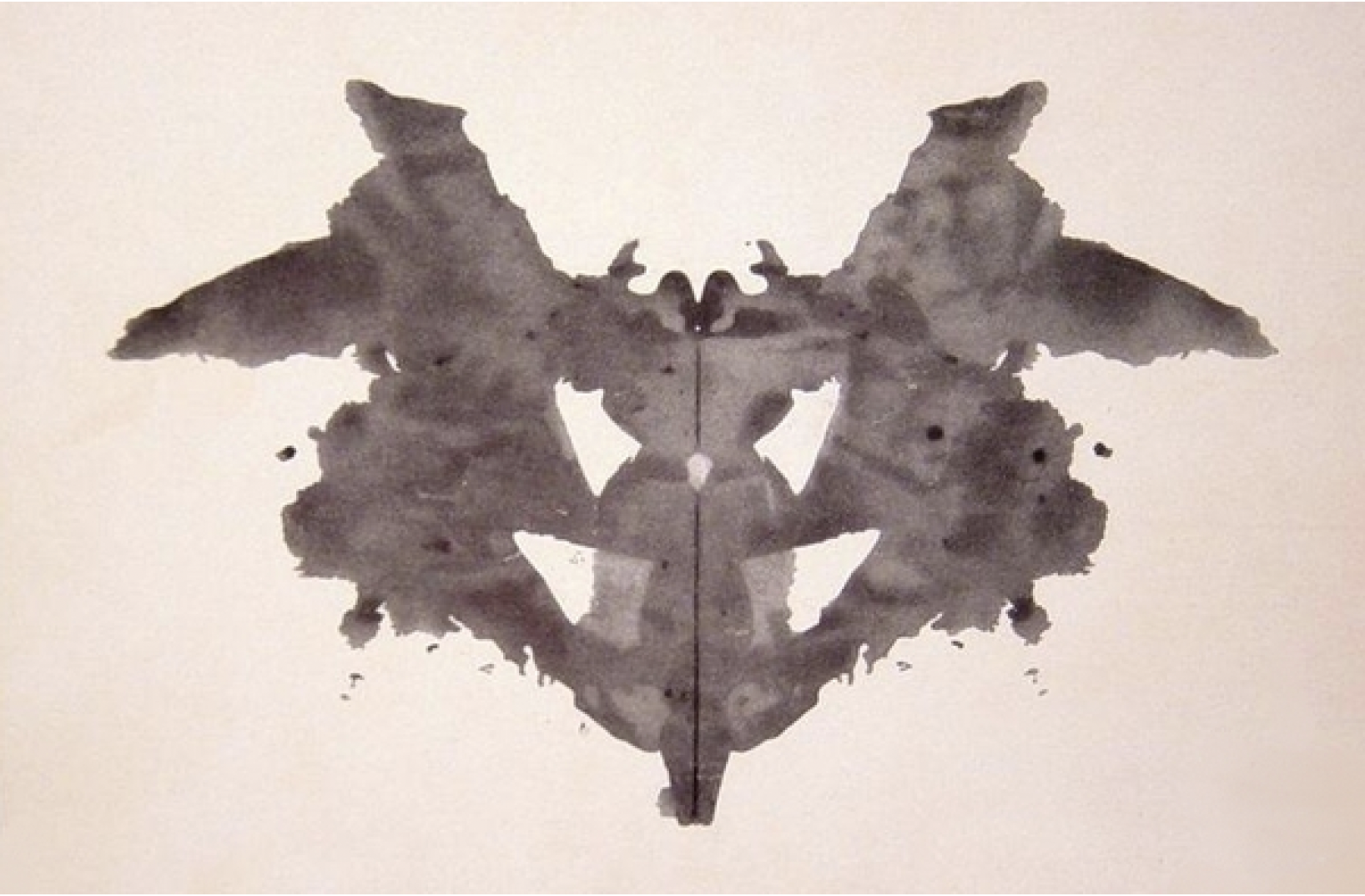
Figure 21. An image from the Rorschach test. What do you see in it?

Let’s take the image illustrated in Figure 21 and use that as our input:

# Load Rorschach image
url = "https://upload.wikimedia.org/wikipedia/commons/7/70/Rorschach_bl
ot_01.jpg"
image = Image.open(urlopen(url)).convert("RGB")

# Generate caption
inputs = blip_processor(image, return_tensors="pt").to(device,
torch.float16)
generated_ids = model.generate(**inputs, max_new_tokens= 20 )
generated_text = blip_processor.batch_decode(generated_ids, skip_special_tokens= True)
generated_text = generated_text[ 0 ].strip()
generated_text

As before, when we inspect the generated_text variable, we can take a look at the caption:

a black and white ink drawing of a bat

I can definitely see how the model would caption this image using such a description. Since this is a Rorschach test, what do you think it says about the model?

Use Case 2: Multimodal Chat-Based Prompting

Although captioning is an important task, we can extend its use case even further. In the previous example, we showed going from one modality, vision (image), to another, text (caption). Instead of following this linear structure, we can try to present both modalities simultaneously by performing what is called visual question answering. In this particular use case, we give the model an image along with a question about that specific image for it to answer. The model needs to process both the image as well as the question at once. To demonstrate, let’s start with the picture of a car and ask BLIP-2 to describe the image. To do so, we first need to preprocess the image as we did a few times before:

# Load an AI-generated image of a supercar
image = Image.open(urlopen(car_path)).convert("RGB")

To perform our visual question answering we need to give BLIP-2 more than just the image, namely the prompt. Without it, the model would generate a caption as it did before. We will ask the model to describe the image we just processed:

# Visual question answering

prompt = "Question: Write down what you see in this picture. Answer:"

# Process both the image and the prompt
inputs = blip_processor(image, text=prompt,
return_tensors="pt").to(device, torch.float16)

# Generate text
generated_ids = model.generate(**inputs, max_new_tokens= 30 )
generated_text = blip_processor.batch_decode(generated_ids, skip_special_tokens= True)
generated_text = generated_text[ 0 ].strip()
generated_text

This gives us the following output:

A sports car driving on the road at sunset

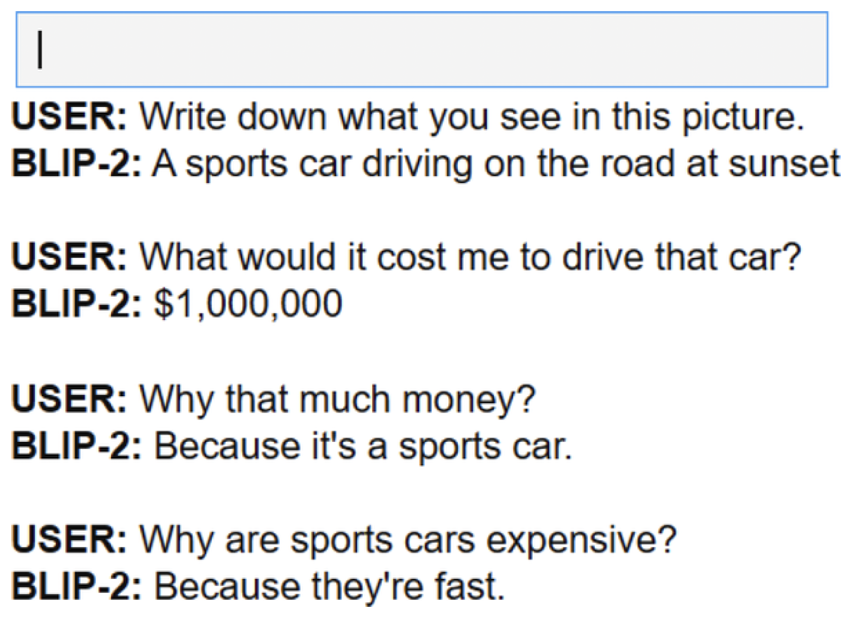
It correctly describes the image. However, this is a rather simple example since our question is essentially asking the model to create a caption. Instead, we can ask follow-up questions in a chat-based manner. To do so, we can give the model our previous conversation, including its answer to our question. We then ask it a follow-up question:

# Chat-like prompting
prompt = "Question: Write down what you see in this picture. Answer: A sports car driving on the road at sunset. Question: What would it cost me to drive that car? Answer:"

# Generate output
inputs = blip_processor(image, text=prompt, return_tensors="pt").to(device, torch.float16)
generated_ids = model.generate(**inputs, max_new_tokens= 30 )
generated_text = blip_processor.batch_decode(generated_ids, skip_special_tokens= True)
generated_text = generated_text[ 0 ].strip()
generated_text

This gives us the following answer:

$1,000,000

$1,000,000 is highly specific! This shows more chat-like behavior from BLIP-2, which allows for some interesting conversations.

Finally, we can make this process a bit smoother by creating an interactive chatbot using ipywidgets, an extension for Jupyter notebooks that allows us to make interactive buttons, input text, etc:

from IPython.display import HTML, display
import ipywidgets as widgets

def text_eventhandler(*args):
    question = args[0]["new"]
    if question:
    args[0]["owner"].value = ""

    # Create prompt
    if not memory:
        prompt = " Question: " + question + "Answer:"
    else :
        template = "Question: {} Answer: {} ."
        prompt = " ".join([template.format(memory[i][0], memory[i][1]) for i in range(len(memory))]) + " Question: " + question + " Answer:"

# Generate text
inputs = blip_processor(image, text=prompt, return_tensors="pt")
inputs = inputs.to(device, torch.float16)
generated_ids = model.generate(**inputs, max_new_tokens=100)
generated_text = blip_processor.batch_decode(generated_ids,skip_special_tokens= True)

generated_text = generated_text[0].strip().split("Question")[0]

# Update memory
memory.append((question, generated_text))

# Assign to output
output.append_display_data(HTML("<b>USER:</b> " + question))
output.append_display_data(HTML("<b>BLIP-2:</b> " +
generated_text))
output.append_display_data(HTML("<br>"))

# Prepare widgets
in_text = widgets.Text()

in_text.continuous_update = **False**
in_text.observe(text_eventhandler, "value")
output = widgets.Output()
memory = []

# Display chat box
display(
    widgets.VBox(children=[output, in_text], layout=widgets.Layout(display="inline-flex", flex_flow="column-reverse"))
)

It seems that we can continue the conversation and ask a bunch of questions. Using this chat-based approach, we essentially created a chatbot that can reason about images!

References

[^fn1]: Jason Wei, Yi Tay, Rishi Bommasani, et al. (2022). Emergent abilities of large language models. arXiv preprint arXiv:2206.07682.
[^fn2]: Alexey Dosovitskiy, Lucas Beyer, Alexander Kolesnikov, et al. (2020). An image is worth 16x16 words: Transformers for image recognition at scale. arXiv preprint arXiv:2010.11929.
[^fn3]: Alec Radford, Jong Wook Kim, Chris Hallacy, et al. (2021). Learning transferable visual models from natural language supervision. In Proceedings of the International Conference on Machine Learning (ICML). PMLR.
[^fn4]: Robin Rombach, Andreas Blattmann, Dominik Lorenz, Patrick Esser, and Björn Ommer. (2022). High-resolution image synthesis with latent diffusion models. In Proceedings of the IEEE/CVF Conference on Computer Vision and Pattern Recognition (CVPR).
[^fn5]: Junnan Li, Dongxu Li, Silvio Savarese, and Steven Hoi. (2023). BLIP-2: Bootstrapping language-image pretraining with frozen image encoders and large language models. In Proceedings of the International Conference on Machine Learning (ICML). PMLR.
[^fn6]: Haotian Liu, Chunyuan Li, Qingyang Wu, and Yizhou Sun. (2024). Visual instruction tuning. In Advances in Neural Information Processing Systems (NeurIPS).
[^fn7]: Hugo Laurençon, Louis Boursier, Renaud Marlet, and Matthieu Cord. (2024). What matters when building vision-language models? arXiv preprint arXiv:2405.02246.
[^fn8]: Roy Schafer. (1954). Psychoanalytic Interpretation in Rorschach Testing: Theory and Application. Grune & Stratton.